吉布斯自由能、化学势与扩散势

The partial Gibbs energy and the Gibbs energy

The partial Gibbs energy, or the chemical potential, is the partial quantity of the Gibbs energy, which means that it is independent of the amount of substance. Generally speaking, the Gibbs energy can be described as a function of temperature, pressure and compositions of components, and thus the chemical potential can be derived from such a mathematical formula. Sometimes, one might feel confused that there exist several different formulas of chemical potential with respect to the Gibbs energy. In this post, two different formulas are to be discussed, respectively.

In the following derivation, the temperature and pressure are assumed as constant.

For Gibbs energy with independent composition

In this context, the Gibbs energy is a function of the solute components, denoted as $1$ to $m-1$, while the $m$-th component is regarded as the solvent.

$G = f(n_1, n_2, ..., n_{m-1})$,

or

$G = N \cdot G_m(x_1, x_2, ..., x_{m-1})$,

where $N$ is the total amount of all the substances, $G_m$ is the mole Gibbs energy, $n_i$ is the amount of the $i$-th component and $x_i$ is the mole fraction of the $i$-th component.

The chemical potential of the $i$-th component, is the partial quantity of the Gibbs energy and that is

$\mu_i = \frac{\partial N G_m}{\partial n_i}.$

In CALPHAD method and other physical models, the mole fraction or the composition is the most common state variable for the fraction of the components. And thus, we have a motivation to substitute the amount, i.e., $n_i$ into fraction, i.e., $x_i$, where chain rule of derivatives should be adopted.

As

$n_i = N \cdot g(x_1, x_2, ..., x_{m-1})$

, we can obtain

$\mu_i = G_m \frac{\partial N }{\partial n_i} + N \sum_{j=1}^{j=m-1}\frac{\partial G_m }{\partial x_j}\frac{\partial x_j }{\partial n_i}$

Take the last part from the equation above and we have

$\frac{\partial x_j }{\partial n_i} = \frac{\partial n_j / N }{\partial n_i}$

Note One should keep in mind that we should not substitute $n_i$ as $N\cdot x_i$, as there is no way to calculate the derivative with respect to fraction number.

Furthermore,

$\frac{\partial x_j }{\partial n_i} = \frac{1}{N^2} (N\frac{\partial n_j}{\partial n_i} - n_j\frac{\partial N}{\partial n_i}).$

Put this result back into the original equation,

$\mu_i = G_m \frac{\partial N }{\partial n_i} + N \sum_{j=1}^{j=m-1}\frac{\partial G_m }{\partial x_j}\frac{1}{N^2} (N\frac{\partial n_j}{\partial n_i} - n_j\frac{\partial N}{\partial n_i})$

Simplify the equation above,

$\mu_i = G_m + \sum_{j=1}^{j=m-1}\frac{\partial G_m }{\partial x_j} (\delta_{ij} - x_j)$

For Gibbs energy with dependent composition

In this context, the Gibbs energy is a function of the solute components, denoted as $1$ to $m-1$, while the $m$-th component is regarded as the solvent.

$G = f(n_1, n_2, ..., n_{m-1}, n_m),$

or

$G = N \cdot G_m(x_1, x_2, ..., x_{m-1}, x_m),$

with a constraint that

$x_1 + x_2 + ... + x_{m-1} + x_m = 1.$

The chemical potential of the $i$-th component, is the partial quantity of the Gibbs energy and that is

$\mu_i = \frac{\partial N G_m}{\partial n_i}.$

In the spirit of the CALPHAD method and other physical models, the mole fraction or the composition is the most common state variable for the fraction of the components. And thus, we have a motivation to substitute the amount, i.e., $n_i$ into fraction, i.e., $x_i$, where chain rule of derivatives should be adopted.

As

$n_i = N \cdot g(x_1, x_2, ..., x_{m-1}, x_m)$

with the previous constraint, and we can obtain

$\mu_i = G_m \frac{\partial N }{\partial n_i} + N \sum_{j=1}^{j=m}\frac{\partial G_m }{\partial x_j}\frac{\partial x_j }{\partial n_i}$

Note It is worthy of noticing that the superscript of the summation has been changed from $m-1$ to $m$.

Take the last part from the equation above and we have

$\frac{\partial x_j }{\partial n_i} = \frac{\partial n_j / N }{\partial n_i}$

Note One should keep in mind that we should not substitute $n_i$ as $N\cdot x_i$, as there is no way to calculate the derivative with respect to fraction number.

Furthermore,

$\frac{\partial x_j }{\partial n_i} = \frac{1}{N^2} (N\frac{\partial n_j}{\partial n_i} - n_j\frac{\partial N}{\partial n_i}).$

Put this result back into the original equation,

$\mu_i = G_m \frac{\partial N }{\partial n_i} + N \sum_{j=1}^{j=m}\frac{\partial G_m }{\partial x_j}\frac{1}{N^2} (N\frac{\partial n_j}{\partial n_i} - n_j\frac{\partial N}{\partial n_i})$

Simplify the equation above,

$\mu_i = G_m + \sum_{j=1}^{j=m}\frac{\partial G_m }{\partial x_j} (\delta_{ij} - x_j)$

Difference between the two formulas of the chemical potential

• For Gibbs energy with independent composition

$\mu_i = G_m + \sum_{j=1}^{j=m-1}\frac{\partial G_m }{\partial x_j} (\delta_{ij} - x_j)$

• For Gibbs energy with dependent composition

$\mu_i = G_m + \sum_{j=1}^{j=m}\frac{\partial G_m }{\partial x_j} (\delta_{ij} - x_j)$

Relation between the chemical potential and the diffusion potential

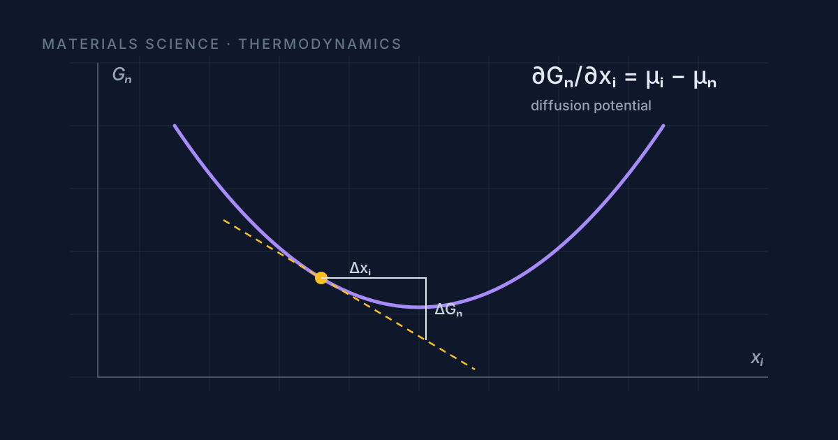
Diffusion potential is one of the most important variables in phase-field modeling. Mathematically, it should be defined as the partial derivative of the mole Gibbs energy.

Note partial derivative of the mole Gibbs energy and the partial quantity of the Gibbs energy are two completely different things.

Considering that the mole Gibbs energy is described with those independent composition variables,

$G_m = G_m(x_1, x_2, ..., x_{m-1})$

the diffusion potential of the $i$-th component with respect to $m$-th component is

$\tilde \mu_i = \frac{\partial G_m}{\partial x_i}$

Note I am writing this to tell that, diffusion potential, is state variable of the solute, which means that a solvent component always exists in this context.

The equation above is really convenient when you have a description of the mole Gibbs energy related to compositions of the solute components. However, CALPHAD technique has adopted the second strategy to demonstrate the relationship between the mole Gibbs energy and composition, which is

$G_m = G_m(x_1, x_2, ..., x_{m-1}, x_m),$

with a constraint that

$x_1 + x_2 + ... + x_{m-1} + x_m = 1.$

Obviously, there is no straight-forward way to compute the derivative of such a formula of the Gibbs energy, as a constraint has been imposed on the function.

Fortunately, we have another definition of the mole Gibbs energy,

$G_m = x_1 \mu_1 + x_2 \mu_2 + ... + x_{m-1} \mu_{m-1} + x_{m} \mu_{m}$

Apply the rule of total derivative to the equation above

$\textrm{d}G_m = \sum_{j=1}^{j=m} \textrm{d}x_j \mu_j + \sum_{j=1}^{j=m} x_j \textrm{d} \mu_j$

According to Gibbs-Duhem equation, we have

$\sum_{j=1}^{j=m} x_j \textrm{d} \mu_j = 0$

and thus

$\textrm{d}G_m = \sum_{j=1}^{j=m} \textrm{d}x_j \mu_j$

Supposing that the $m$-th is the solvent component, the composition of the solvent can be substituted with those of the solutes,

$\textrm{d}G_m = \sum_{j=1}^{j=m-1} \textrm{d}x_j \mu_j + \textrm{d} (1 - \sum_{j=1}^{j=m-1} x_j) \mu_m$

because

$x_m = 1 - \sum_{j=1}^{j=m-1} x_j$

Consequently, all the composition variables in the equation above become independent, and we know

$\frac{\partial G_m}{\partial x_i} = \mu_i - \mu_{m}$

according to the properties of the total derivative.

计算理想固溶体的吉布斯自由能、化学势和扩散势

void func_compenstate_multicomponent(const double *x, double *f, int cnum)
{
    double T = x[cnum-1]; // the last element is temperature
    double vars[cnum];
    double v = 0;
    for (int i = 0; i < cnum-1; i++)
    {
        vars[i] = x[i] < 1.0e-6 ? 1.0e-6 : (x[i] > 1.0 - 1.0e-6 ? 1.0 - 1.0e-6 : x[i]);
        v += vars[i];
    }
    vars[cnum-1] = 1.0 - v;

    double gm = 0;
    for (int ci=0; ci<cnum; ci++)
    {
        gm += vars[ci] * log(vars[ci]);
    }
    gm = 8.31451 * T * gm;
    f[0] = gm;

    double partial_gm[cnum];
    for (int ci=0; ci<cnum; ci++)
    {
        partial_gm[ci] = 8.31451 * T * (log(vars[ci]) + 1);
    }

    double sum_partial_gm = 0;
    for (int ci=0; ci<cnum; ci++)
    {
        sum_partial_gm += partial_gm[ci] * vars[ci];
    }

    double mus[cnum];
    for (int ci=0; ci<cnum; ci++)
    {
        mus[ci] = gm + partial_gm[ci] - sum_partial_gm;
    }

    for (int ci=0; ci<cnum-1; ci++)
    {
        f[ci+1] = mus[ci] - mus[cnum-1];
    }
}

void func_compenstate_quaternary(const double *x, double *f)
{
    func_compenstate_multicomponent(x, f, 4);
}